Building CLIP From Scratch: Unfolding Story Behind Pixels

Table of contents

• Understanding CLIP’s Training Objective
• Model Architecture
• Positional Embedding
• Attention Head
• Multi-Head Attention
• Transformer Encoder
• Image Encoder
• Text Encoder
• Dataset Preparation
• Tokenization
• CLIP Model
• Training
• Hyperparameter Tuning
• Evaluation and Inference with Gradio
• CLIP Inference with Gradio
• Conclusion
• References

Contrastive Language-Image Pre-training (CLIP) was developed by OpenAI and first introduced in the paper “Learning Transferable Visual Models From Natural Language Supervision” in 2021. It was designed to improve zero-shot learning in computer vision by training on a vast number of image-text pairs from the internet.

The conventional approach to visual perception has long followed a standard formula:

1. Pre-train a CNN on large labeled datasets (typically ImageNet).
2. Fine-tune on specific tasks with smaller datasets.

While this approach has produced impressive results, it has significant limitations:

• Requires extensive manual annotation
• Limited by the scope of pre-defined classes
• Lacks flexibility for new tasks

In 2016, Li et al. pioneered the use of natural language for visual prediction, achieving 11.4% zero-shot accuracy on ImageNet and Flickr comments. Mahajan et al. (2018) demonstrated that using Instagram hashtags for pre-training could significantly improve model performance, increasing ImageNet accuracy by over 5%.

OpenAI’s introduction of CLIP in 2021 revolutionized the field by training 400 million image-text pairs. Unlike its predecessors, CLIP combined a powerful vision encoder with a robust text encoder, trained through contrastive learning. This approach enabled zero-shot learning across various tasks, eliminating the need for task-specific training.

Understanding CLIP’s Training Objective

Early approaches to training vision-language models, such as Mahajan et al. (2018) and Xie et al. (2020), required extensive computational resources — ranging from 19 GPU years to 33 TPUv3 core years. Initially, the authors of CLIP attempted to train an image CNN and a transformer-based text model from scratch to predict image captions. However, this approach proved inefficient, as the language model struggled to generalize beyond memorizing hashtags and comments.

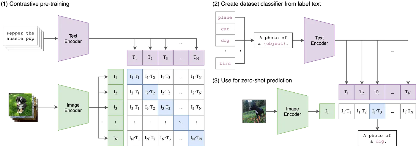
To overcome these challenges, CLIP adopts a contrastive learning objective, significantly improving efficiency. The model is trained on N image-text pairs, where both the image and text are encoded into a shared multimodal embedding space. The goal is to maximize the cosine similarity between correct image-text pairs while minimizing the similarity between incorrect pairs. This results in a more scalable and generalizable model that can recognize visual concepts without task-specific fine-tuning.

By utilizing contrastive learning, CLIP efficiently aligns visual and textual representations, enabling robust zero-shot classification and transfer learning across different domains.

Model Architecture

CLIP employs two different backbones for its image encoder — ResNet-50 and Vision Transformer (ViT) — while using a transformer-based text encoder. The largest ResNet variant, RN50x64, required 18 days of training on 592 V100 GPUs, whereas the largest Vision Transformer variant was trained in 12 days on 256 V100 GPUs.

The model is instantiated with attributes such as embed_dim, which defines the embedding space dimensions, and width and layers, which specify the architecture’s depth. If the vision_layers attribute is provided as a tuple or list, ResNet is used as the image encoder’s backbone; otherwise, the Visual Transformer is selected.

Let’s walk through how we can build and train CLIP from scratch. This workflow consists of several key components:

1. Positional Embedding
2. Attention Head
3. Multi-Head Attention
4. Transformer Encoder
5. Image Encoder
6. Text Encoder
7. Dataset Preparation
8. Tokenization
9. CLIP Model
10. Training
11. Hyper-parameter Tuning
12. Model Evaluation and Inference with Gradio

Import Required Dependencies

First, let’s set up all the necessary imports that are required for our implementation.

import torch
import torch.nn as nn
from torch.utils.data import Dataset, DataLoader
from torch.optim import Adam

import torchvision.transforms as T
from PIL import Image

import numpy as np
import pandas as pd
import os
from tqdm import tqdm

import matplotlib.pyplot as plt
import gradio as gr
import plotly.graph_objects as go

We are using PyTorch as the foundation of our implementation, providing efficient tensor operations.

import torch
import torch.nn as nn

We are working with DataSet and DataLoader modules for efficient data loading and batch processing.

from torch.utils.data import Dataset, DataLoader

Here, in our implementation, we are using an Adam optimizer, so let’s import it.

from torch.optim import Adam

Also, we are using torchvision.transforms module that provides transformations like data resizing, normalization, and augmentation.

import torchvision.transforms as T

For visualizing the CLIP model’s performance, we are using a couple of visualization packages: Matplotlib for basic training plots, while Gradio enables us to build a web user interface for model evaluation, and Plotly provides interactive-dynamic visualizations.

import matplotlib.pyplot as plt
import gradio as gr
import plotly.graph_objects as go

Positional Embedding

We define a PositionalEmbedding class using PyTorch, which introduces positional information to input sequences. Since transformers lack inherent order awareness, positional embeddings help sequence order, allowing the model to differentiate between token positions.

class PositionalEmbedding(nn.Module):
    def __init__(self, width, max_seq_length):
        super().__init__()
        pe = torch.zeros(max_seq_length, width)
        for pos in range(max_seq_length):
            for i in range(width):
                if i % 2 == 0:
                    pe[pos][i] = np.sin(pos/(10000 ** (i/width)))
                else:
                    pe[pos][i] = np.cos(pos/(10000 ** ((i-1)/width)))
        self.register_buffer('pe', pe.unsqueeze(0))

    def forward(self, x):
        return x + self.pe

At first, a positional embedding matrix, pe, is created and initialized to zeros.

pe = torch.zeros(max_seq_length, width)

Each position is assigned unique values using sinusoidal functions — sine for even indices and cosine for odd indices. It ensures smooth transitions between positions, which helps the model learn relative positional relationships.

for pos in range(max_seq_length):
    for i in range(width):
        if i % 2 == 0:
            pe[pos][i] = np.sin(pos/(10000 ** (i/width)))
        else:
            pe[pos][i] = np.cos(pos/(10000 ** ((i-1)/width)))

Also, we stored these embeddings as a buffer, ensuring it is not updated during training.

self.register_buffer('pe', pe.unsqueeze(0))

In the forward pass, the computed positional embeddings are added to the input, adding position-related information without changing the model’s learned weights.

def forward(self, x):
    return x + self.pe

Attention Head

Next up in our workflow is defining the AttentionHead class, which forms the core of the self-attention mechanism in Transformers.

Let’s understand attention first:

Attention is a mechanism that allows models to dynamically focus on different parts of an input sequence, enabling them to capture long-range dependencies effectively.

class AttentionHead(nn.Module):
    def __init__(self, width, head_size):
        super().__init__()
        self.head_size = head_size
        self.query = nn.Linear(width, head_size)
        self.key = nn.Linear(width, head_size)
        self.value = nn.Linear(width, head_size)

    def forward(self, x, mask=None):
        B, T, C = x.shape  # batch, sequence length, channels
        Q = self.query(x)  # (B, T, head_size)
        K = self.key(x)    # (B, T, head_size)
        V = self.value(x)  # (B, T, head_size)
        
        # Compute attention scores
        attention = Q @ K.transpose(-2, -1)  # (B, T, T)
        attention = attention / (self.head_size ** 0.5)
        
        # Create attention mask
        if mask is not None:
            # Create a mask for attention scores
            # mask shape: (B, T) -> attention_mask shape: (B, T, T)
            attention_mask = mask.unsqueeze(1).expand(-1, T, -1)
            attention = attention.masked_fill(attention_mask == 0, float('-inf'))
        
        attention = torch.softmax(attention, dim=-1)
        return attention @ V

In our implementation, we defined an AttentionHead class that captures token relationships through query (Q), key (K), and value (V) transformations.

At first, we declare three linear layers:

• Query (Q): Determines what the current token is looking for.
• Key (K): Represents how relevant each token is to the query.
• Value (V): Holds the actual token information to be weighted.

Each transformation allows multiple heads to focus on different aspects of an input sequence.

class AttentionHead(nn.Module):
    def __init__(self, width, head_size):
        super().__init__()
        self.head_size = head_size
        self.query = nn.Linear(width, head_size)
        self.key = nn.Linear(width, head_size)
        self.value = nn.Linear(width, head_size)

In the forward pass, we extract the batch size, sequence length, and embedding dimension and compute query (Q), key (K), and value (V) projections.

def forward(self, x, mask=None):
    B, T, C = x.shape  # batch, sequence length, channels
    Q = self.query(x)  # (B, T, head_size)
    K = self.key(x)    # (B, T, head_size)
    V = self.value(x)  # (B, T, head_size)

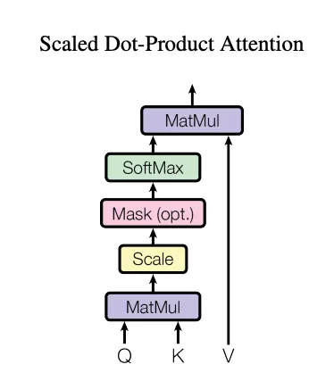
After calculating the query, key, and value, we calculate attention scores using scaled-dot product attention, which measures token similarity.

As discussed here, the scaled-dot product attention equation is written as:

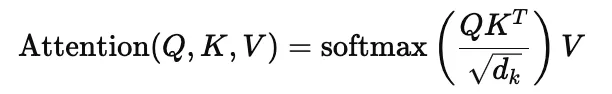
Here Q (Query), K (Key), and V (Value) are linear projections of the input, and dk is the key dimension.

The dot product between queries and keys measure similarity, and the softmax normalizes these scores into a probability distribution, deciding how much focus should be given to each token.

# Compute attention scores
attention = Q @ K.transpose(-2, -1)  # (B, T, T)
attention = attention / (self.head_size ** 0.5)

If the mask is provided (e.g., for casual attention in autoregressive models), it is used to prevent attention to certain positions, ensuring the model only attends to valid tokens.

# Create attention mask
if mask is not None:
    # Create a mask for attention scores
    # mask shape: (B, T) -> attention_mask shape: (B, T, T)
    attention_mask = mask.unsqueeze(1).expand(-1, T, -1)
    attention = attention.masked_fill(attention_mask == 0, float('-inf'))

These scores are passed through softmax function, converting them into normalized attention weights. And we return the weighted sum of values (V) representing context-aware token embeddings.

attention = torch.softmax(attention, dim=-1)
return attention @ V

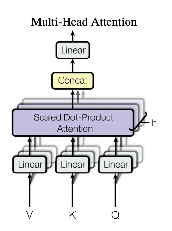
Multi-Head Attention

It is a key component in Transformer architecture that enhances self-attention using multiple independent attention heads. Each head computes attention separately, focusing on different relationships within the input, and the outputs are then concatenated and transformed.

class MultiHeadAttention(nn.Module):
    def __init__(self, width, n_heads):
        super().__init__()
        self.head_size = width // n_heads
        self.heads = nn.ModuleList([AttentionHead(width, self.head_size) for _ in range(n_heads)])
        self.W_o = nn.Linear(width, width)

    def forward(self, x, mask=None):
        out = torch.cat([head(x, mask=mask) for head in self.heads], dim=-1)
        return self.W_o(out)

While initializing, we divide the embedding dimension equally among the number of heads and create multiple attention heads. Next, we use a final transformation W_o, which projects concatenated outputs of all attention heads back to the original embedding dimension.

def __init__(self, width, n_heads):
    super().__init__()
    self.head_size = width // n_heads
    self.heads = nn.ModuleList([AttentionHead(width, self.head_size) for _ in range(n_heads)])
    self.W_o = nn.Linear(width, width)

In the forward method, we pass an input through each attention head separately and concatenate the outputs of all heads along the last dimension.

And we return a linear projection W_o that combines the information from different heads.

def forward(self, x, mask=None):
    out = torch.cat([head(x, mask=mask) for head in self.heads], dim=-1)
    return self.W_o(out)

Transformer Encoder

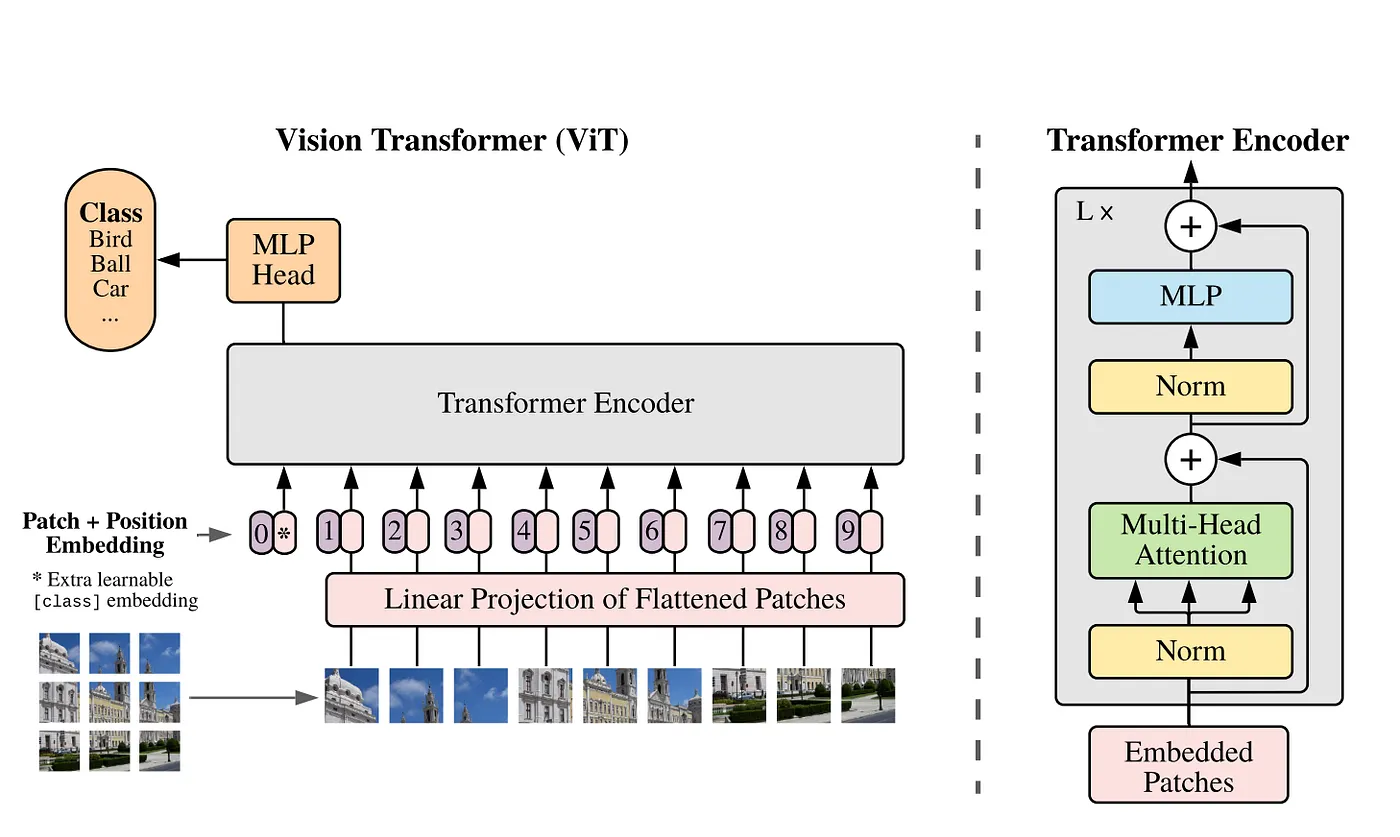
With multi-head attention in place, let’s move to the Transformer Encoder, which is a fundamental component of models like BERT and Vision Transformers (ViTs).

It is responsible for processing input sequences while capturing contextual dependencies.

class TransformerEncoder(nn.Module):
    def __init__(self, width, n_heads, r_mlp=4):
        super().__init__()
        self.width = width
        self.n_heads = n_heads
        self.ln1 = nn.LayerNorm(width)
        self.mha = MultiHeadAttention(width, n_heads)
        self.ln2 = nn.LayerNorm(width)
        self.mlp = nn.Sequential(
            nn.Linear(width, width*r_mlp),
            nn.GELU(),
            nn.Linear(width*r_mlp, width)
        )

    def forward(self, x, mask=None):
        x = x + self.mha(self.ln1(x), mask=mask)
        x = x + self.mlp(self.ln2(x))
        return x

The class initializes with layer normalizations (ln1 and ln2), which stabilizes activations and ensures smoother training. Next, it applies Multi-Head Attention (MHA), which allows the encoder to capture contextual dependencies across the input sequence by attending to different parts of the data simultaneously.

def __init__(self, width, n_heads, r_mlp=4):
    super().__init__()
    self.width = width
    self.n_heads = n_heads
    self.ln1 = nn.LayerNorm(width)
    self.mha = MultiHeadAttention(width, n_heads)
    self.ln2 = nn.LayerNorm(width)
    self.mlp = nn.Sequential(
            nn.Linear(width, width*r_mlp),
            nn.GELU(),
            nn.Linear(width*r_mlp, width)
        )

Additionally, a feedforward network (MLP) expands the feature dimension, applies the GELU activation function, and projects it back to the original width.

The forward method processes input tensor x by first applying layer normalization (ln1), followed by multi-head attention (MHA) to capture contextual relationships. The result is added back to the input tensor x via a residual connection.

def forward(self, x, mask=None):
    x = x + self.mha(self.ln1(x), mask=mask)
    x = x + self.mlp(self.ln2(x))
    return x

Next, Layer Normalization (ln2) is applied, followed by an MLP block for further feature refinement.

Image Encoder

It is responsible for transforming input images into a high-dimensional representation that can be used for downstream tasks such as vision-language modeling.

class ImageEncoder(nn.Module):
    def __init__(self, width, img_size, patch_size, n_channels, n_layers, n_heads, emb_dim):
        super().__init__()
        assert img_size[0] % patch_size[0] == 0 and img_size[1] % patch_size[1] == 0
        
        self.n_patches = (img_size[0] * img_size[1]) // (patch_size[0] * patch_size[1])
        self.max_seq_length = self.n_patches + 1
        
        self.linear_project = nn.Conv2d(n_channels, width, kernel_size=patch_size, stride=patch_size)
        self.cls_token = nn.Parameter(torch.randn(1, 1, width))
        self.positional_embedding = PositionalEmbedding(width, self.max_seq_length)
        self.encoder = nn.ModuleList([TransformerEncoder(width, n_heads) for _ in range(n_layers)])
        self.projection = nn.Parameter(torch.randn(width, emb_dim))

    def forward(self, x):
        x = self.linear_project(x)
        x = x.flatten(2).transpose(1, 2)
        x = torch.cat((self.cls_token.expand(x.size()[0], -1, -1), x), dim=1)
        x = self.positional_embedding(x)
        
        for encoder_layer in self.encoder:
            x = encoder_layer(x)
        
        x = x[:, 0, :]
        x = x @ self.projection
        return x / torch.norm(x, dim=-1, keepdim=True)

The encoder initializes by ensuring that the image dimension is perfectly divisible by the patch size (patch_size). Next, it computes the total number of image patches and defines the maximum sequence length by adding a classification token.

def __init__(self, width, img_size, patch_size, n_channels, n_layers, n_heads, emb_dim):
    super().__init__()
    assert img_size[0] % patch_size[0] == 0 and img_size[1] % patch_size[1] == 0
        
    self.n_patches = (img_size[0] * img_size[1]) // (patch_size[0] * patch_size[1])
    self.max_seq_length = self.n_patches + 1

The patch embeddings I performed used a 2D convolution that maps input image patches to a lower-dimensional space with (width) channels. Also, a positional embedding is applied to retain spatial information.

self.linear_project = nn.Conv2d(n_channels, width, kernel_size=patch_size, stride=patch_size)
self.cls_token = nn.Parameter(torch.randn(1, 1, width))
self.positional_embedding = PositionalEmbedding(width, self.max_seq_length)

---

The encoder stack consists of multiple Transformer encoder layers, which refine patch representations through self-attention. Finally, a projection layer maps the encoded features into the final embedding.

self.encoder = nn.ModuleList([TransformerEncoder(width, n_heads) for _ in range(n_layers)])
self.projection = nn.Parameter(torch.randn(width, emb_dim))

In the forward pass, the image is first transformed into patch embeddings using a convolutional layer, then flattened and transposed to match the Transformer input format. A classification token cls_token is appended to serve as a global representation of the image. Next, positional embeddings are added to retain spatial structure.

def forward(self, x):
    x = self.linear_project(x)
    x = x.flatten(2).transpose(1, 2)
    x = torch.cat((self.cls_token.expand(x.size()[0], -1, -1), x), dim=1)
    x = self.positional_embedding(x)

The patch embeddings are then sequentially processed through multiple Transformer Encoder layers.

for encoder_layer in self.encoder:
    x = encoder_layer(x)

The final image representation is extracted from the CLS token’s output, followed by a projection step that maps it to the desired embedding dimension. The resulting vector is normalized, ensuring stable representations.

x = x[:, 0, :]
x = x @ self.projection
return x / torch.norm(x, dim=-1, keepdim=True)

Text Encoder

The Text Encoder converts input text into a dense, high-dimensional embedding, enabling effective representation learning for language understanding.

class TextEncoder(nn.Module):
    def __init__(self, vocab_size, width, max_seq_length, n_heads, n_layers, emb_dim):
        super().__init__()
        self.max_seq_length = max_seq_length
        self.encoder_embedding = nn.Embedding(vocab_size, width)
        self.positional_embedding = PositionalEmbedding(width, max_seq_length)
        self.encoder = nn.ModuleList([TransformerEncoder(width, n_heads) for _ in range(n_layers)])
        self.projection = nn.Parameter(torch.randn(width, emb_dim))
        self.width = width

    def forward(self, text, mask=None):
        batch_size = text.shape[0]
        
        # [batch_size, seq_len, width]
        x = self.encoder_embedding(text)
        x = self.positional_embedding(x)
        
        # Apply transformer layers
        for encoder_layer in self.encoder:
            x = encoder_layer(x, mask=mask)
        
        # Extract features from the CLS token (first token)
        x = x[:, 0, :]  # Take the first token (CLS token) from each sequence
        
        # Project to embedding dimension and normalize
        x = x @ self.projection
        return x / torch.norm(x, dim=-1, keepdim=True)

The model begins with an embedding layer that maps input tokens to a width-dimensional space. A positional embedding is added to retain token order. The text is then processed through a stack of Transformer Encoder layers, capturing long-range dependencies. Finally, a learnable projection maps the encoded features to the desired embedding dimension emb_dim.

def __init__(self, vocab_size, width, max_seq_length, n_heads, n_layers, emb_dim):
    super().__init__()
    self.max_seq_length = max_seq_length
    self.encoder_embedding = nn.Embedding(vocab_size, width)
    self.positional_embedding = PositionalEmbedding(width, max_seq_length)
    self.encoder = nn.ModuleList([TransformerEncoder(width, n_heads) for _ in range(n_layers)])
    self.projection = nn.Parameter(torch.randn(width, emb_dim))
    self.width = width

In the forward method, the input text is first embedded and enriched with positional information. It then passes through multiple Transformer Encoder layers, refining token representations. The CLS token’s output is extracted as the final sentence representation. A projection step follows, and the output is L2-normalized to ensure stable feature representations.

def forward(self, text, mask=None):
    batch_size = text.shape[0]
        
    # [batch_size, seq_len, width]
    x = self.encoder_embedding(text)
    x = self.positional_embedding(x)
    
    # Apply transformer layers
    for encoder_layer in self.encoder:
        x = encoder_layer(x, mask=mask)
    
    # Extract features from the CLS token (first token)
    x = x[:, 0, :]  # Take the first token (CLS token) from each sequence
    
    # Project to embedding dimension and normalize
    x = x @ self.projection
    return x / torch.norm(x, dim=-1, keepdim=True)

Dataset Preparation

For training, we will use the Flickr8K dataset, which consists of 8,000 images, each accompanied by multiple textual captions. The dataset will be preprocessed and loaded using a custom PyTorch Dataset class.

class FlickrDataset(Dataset):
    def __init__(self, df, image_path, transform=None):
        self.df = df
        self.image_path = image_path
        self.transform = transform or T.Compose([
            T.Resize((224, 224)),
            T.ToTensor(),
            T.Normalize(mean=[0.485, 0.456, 0.406], std=[0.229, 0.224, 0.225])
        ])
        
        self.image_groups = df.groupby('image')
        self.unique_images = list(self.image_groups.groups.keys())

    def __len__(self):
        return len(self.unique_images)

    def __getitem__(self, idx):
        image_name = self.unique_images[idx]
        captions = self.image_groups.get_group(image_name)['caption'].tolist()
        caption = np.random.choice(captions)
        image = Image.open(os.path.join(self.image_path, image_name)).convert('RGB')
        image = self.transform(image)
        tokens, mask = tokenizer(caption)
        return {'image': image, 'caption': tokens, 'mask': mask, 'raw_caption': caption}

The dataset is initialized with a DataFrame containing image-caption pairs and the respected image directory path. Now, transformations are applied, including resizing, normalization, and tensor conversion. Then images are grouped to allow considering multiple captions for each unique image.

def __init__(self, df, image_path, transform=None):
    self.df = df
    self.image_path = image_path
    self.transform = transform or T.Compose([
        T.Resize((224, 224)),
        T.ToTensor(),
        T.Normalize(mean=[0.485, 0.456, 0.406], std=[0.229, 0.224, 0.225])
    ])
    
    self.image_groups = df.groupby('image')
    self.unique_images = list(self.image_groups.groups.keys())

The length of the dataset corresponds to the number of unique images, ensuring that each image is accessed individually rather than counting all caption duplicates.

def __len__(self):
    return len(self.unique_images)

Given an index, the __getitem__ method retrieves an image filename and selects a corresponding caption. The image is loaded, converted to RGB, and transformed for model input. The caption is tokenized using a predefined tokenizer, returning the token sequence and an attention mask. The final output is a dictionary containing:

The processed image The tokenized caption The attention mask, and The raw caption text

def __getitem__(self, idx):
    image_name = self.unique_images[idx]
    captions = self.image_groups.get_group(image_name)['caption'].tolist()
    caption = np.random.choice(captions)
    image = Image.open(os.path.join(self.image_path, image_name)).convert('RGB')
    image = self.transform(image)
    tokens, mask = tokenizer(caption)
    return {'image': image, 'caption': tokens, 'mask': mask, 'raw_caption': caption}

Tokenization

The tokenizer function is responsible for encoding text into a numerical format suitable for deep learning models and decoding tokenized sequences back into text. It ensures that input text adheres to a fixed sequence length while maintaining important structural elements like start and end tokens.

def tokenizer(text, encode=True, mask=None, max_seq_length=77): 
    if encode:
        # Add start and end tokens
        out = chr(2) + text + chr(3)
        
        # Truncate if longer than max_seq_length
        if len(out) > max_seq_length:
            out = out[:max_seq_length-1] + chr(3) 
        
        # Pad with zeros if shorter than max_seq_length
        out = out + "".join([chr(0) for _ in range(max_seq_length - len(out))])
        
        # Convert to tensor
        out = torch.IntTensor(list(out.encode("utf-8")))
        
        # Create mask (1s for actual tokens, 0s for padding)
        n_actual_tokens = len(text) + 2  # +2 for start and end tokens
        n_actual_tokens = min(n_actual_tokens, max_seq_length)

        # Create a 1D mask tensor
        mask = torch.zeros(max_seq_length, dtype=torch.long)
        mask[:n_actual_tokens] = 1  # Set 1s for actual tokens
        
    else:
        # Decoding
        if mask is None:
            raise ValueError("Mask is required for decoding")
        
        # Convert back to text, removing start and end tokens
        out = [chr(x) for x in text[1:len(mask.nonzero())]]
        out = "".join(out)
        mask = None

    return out, mask

During encoding, the function first adds special tokens: a start token (chr(2)) at the beginning and an end token (chr(3)) at the end of the text.

If the text length exceeds the defined max_seq_length, it is truncated while ensuring the end token is retained. If the text is shorter than the required length, zero-padding is applied to maintain a uniform input size.

if encode:
    # Add start and end tokens
    out = chr(2) + text + chr(3)
    
    # Truncate if longer than max_seq_length
    if len(out) > max_seq_length:
        out = out[:max_seq_length-1] + chr(3) 
    
    # Pad with zeros if shorter than max_seq_length
    out = out + "".join([chr(0) for _ in range(max_seq_length - len(out))])

The processed text is then converted into a tensor using UTF-8 encoding, allowing the model to interpret it numerically. Additionally, an attention mask is generated, marking actual tokens with 1s and padded positions with 0s, helping the model distinguish between meaningful input and padding.

# Convert to tensor
out = torch.IntTensor(list(out.encode("utf-8")))

# Create mask (1s for actual tokens, 0s for padding)
n_actual_tokens = len(text) + 2  # +2 for start and end tokens
n_actual_tokens = min(n_actual_tokens, max_seq_length)

# Create a 1D mask tensor
mask = torch.zeros(max_seq_length, dtype=torch.long)
mask[:n_actual_tokens] = 1  # Set 1s for actual tokens

For decoding, the function reconstructs the text by converting tokenized numerical sequences back into readable format. The start and end tokens are removed, and the original text is retrieved. A mask is required during decoding to determine valid token positions and prevent unnecessary processing of padding elements.

# Decoding
# Convert back to text, removing start and end tokens
out = [chr(x) for x in text[1:len(mask.nonzero())]]
out = "".join(out)
mask = None

By implementing this tokenizer, textual data is efficiently structured and aligned for our model architecture, ensuring consistency in sequence-based learning.

CLIP Model

The CLIP class is a multimodal learning model that processes both images and text, enabling them to be mapped into a shared embedding space. It integrates an ImageEncoder for processing visual data and an TextEncoder for handling textual input. The architecture allows these two different modalities to interact meaningfully, making it suitable for tasks like:

• Zero-Shot Image Classification
• Semantic Image Retrieval
• Image Ranking
• Reverse Image Search
• Image Capturing, etc.

class CLIP(nn.Module):
    def __init__(self, config):
        super().__init__()
        self.image_encoder = ImageEncoder(
            config['width'],
            config['img_size'],
            config['patch_size'],
            config['n_channels'],
            config['vit_layers'],
            config['vit_heads'],
            config['emb_dim']
        )
        self.text_encoder = TextEncoder(
            config['vocab_size'],
            config['text_width'],
            config['max_seq_length'],
            config['text_heads'],
            config['text_layers'],
            config['emb_dim']
        )
        self.temperature = nn.Parameter(torch.ones([]) * np.log(1 / 0.07))
        self.device = torch.device("cuda" if torch.cuda.is_available() else "cpu")

    def forward(self, image, text, mask=None):
        # Move mask to the same device as the model
        if mask is not None:
            mask = mask.to(self.device)
            
        image_features = self.image_encoder(image)
        text_features = self.text_encoder(text, mask=mask)
        
        # Compute similarity
        logits = (image_features @ text_features.transpose(-2, -1)) * torch.exp(self.temperature)
        
        # Compute loss
        labels = torch.arange(logits.shape[0], device=self.device)
        loss_i = nn.functional.cross_entropy(logits.transpose(-2, -1), labels)
        loss_t = nn.functional.cross_entropy(logits, labels)
        
        return (loss_i + loss_t) / 2

In the initialization method __init__, the image encoder extracts feature representations from images, breaking them down into patches and processing them through multiple transformer layers.

self.image_encoder = ImageEncoder(
                          config['width'],
                          config['img_size'],
                          config['patch_size'],
                          config['n_channels'],
                          config['vit_layers'],
                          config['vit_heads'],
                          config['emb_dim']
                        )

Similarly, the text encoder converts input text into meaningful embeddings.

self.text_encoder = TextEncoder(
                        config['vocab_size'],
                        config['text_width'],
                        config['max_seq_length'],
                        config['text_heads'],
                        config['text_layers'],
                        config['emb_dim']
                    )

In the forward pass, images and text are encoded separately using their respective encoders.

image_features = self.image_encoder(image)
text_features = self.text_encoder(text, mask=mask)

The resulting feature vectors are then used to compute a similarity matrix between all image-text pairs using a dot product, scaled by the exponential of the temperature parameter. This similarity matrix serves as the foundation for contrastive learning.

# Compute similarity
logits = (image_features @ text_features.transpose(-2, -1)) * torch.exp(self.temperature)

To train the model, cross-entropy loss is applied to ensure that correct image-text pairs are ranked higher than incorrect ones.

The final loss is an average of two objectives: aligning images with their corresponding texts and vice versa.

# Compute loss
labels = torch.arange(logits.shape[0], device=self.device)
loss_i = nn.functional.cross_entropy(logits.transpose(-2, -1), labels)
loss_t = nn.functional.cross_entropy(logits, labels)

return (loss_i + loss_t) / 2

Training

The CLIP model will be trained using a contrastive loss function, which ensures that images and their corresponding text descriptions are mapped to similar representations in the embedding space.

def train_clip(model, train_loader, optimizer, device, epochs=30):
    model.train()
    best_loss = float('inf')
    
    for epoch in range(epochs):
        total_loss = 0
        progress_bar = tqdm(train_loader, desc=f'Epoch {epoch+1}/{epochs}')
        
        for batch in progress_bar:
            images = batch['image'].to(device)
            captions = batch['caption'].to(device)
            masks = batch['mask'].to(device)
            
            loss = model(images, captions, masks)
            
            optimizer.zero_grad()
            loss.backward()
            optimizer.step()
            
            total_loss += loss.item()
            progress_bar.set_postfix({'loss': loss.item()})
        
        avg_loss = total_loss / len(train_loader)

In the training loop, the model is set to training model.train(), ensuring that parameters are updated during back-propagation.

The CLIP model’s forward pass computes the contrastive loss, which measures how well the model aligns image-text pairs. The optimizer is then used to update the model’s weights. And this function also keeps track of the total loss across batches.

loss = model(images, captions, masks)
           
optimizer.zero_grad()
loss.backward()
optimizer.step()

total_loss += loss.item()

After completing an epoch, it calculates and prints the average loss, helping monitor the model’s improvement over time.

avg_loss = total_loss / len(train_loader)
print(f'Epoch [{epoch+1}/{epochs}], Average Loss: {avg_loss:.4f}')

Hyperparameter Tuning

The provided configuration defines the architectural and training parameters for the CLIP model.

emb_dim: 256
width: 768
img_size: (224, 224)
patch_size: (16, 16)
n_channels: 3
vit_layers: 6
vit_heads: 8
vocab_size: 25000
text_width: 512
max_seq_length: 77
text_heads: 8
text_layers: 6
batch_size: 32
learning_rate: 1e-4
epochs: 10

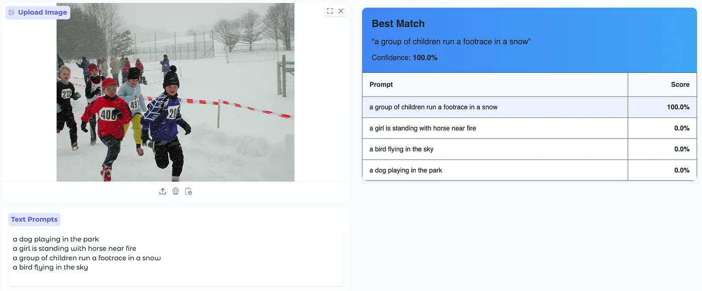
Evaluation and Inference with Gradio

Once trained, this model can be used to analyze images. The function get_image_text_similarity performs inference with the trained CLIP model, computing the similarity between an input image and text prompts.

def get_image_text_similarity(model, image_tensor, text_tokens, text_masks):
    """Calculate similarity between image and text prompts."""
    with torch.no_grad():
        device = next(model.parameters()).device
        image_tensor = image_tensor.to(device)
        text_tokens = text_tokens.to(device)
        text_masks = text_masks.to(device)
        
        # Get embeddings
        image_features = model.image_encoder(image_tensor)
        text_features = model.text_encoder(text_tokens, mask=text_masks)
        
        # Compute similarities and probabilities
        similarities = (image_features @ text_features.transpose(-2, -1)).squeeze(0)
        similarities = similarities * torch.exp(model.temperature)
        probabilities = torch.nn.functional.softmax(similarities, dim=-1)
        
        return probabilities.cpu().numpy()

The function extracts image and text embeddings using the respective encoders and computes their similarity via the dot product. This score is scaled using the learned temperature parameter to adjust distribution sharpness.

Finally, a softmax function normalizes the scores into probabilities, indicating how well the image matches different text prompts.

The Gradio-based UI allows to:

• Upload an image and input multiple text prompts.
• Compute similarity scores between the image and text inputs.
• Display results in a structured format with confidence scores.

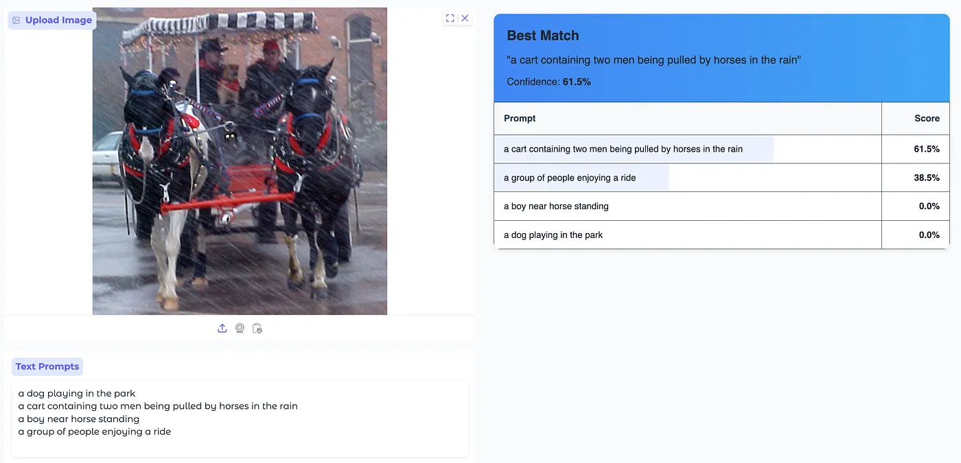
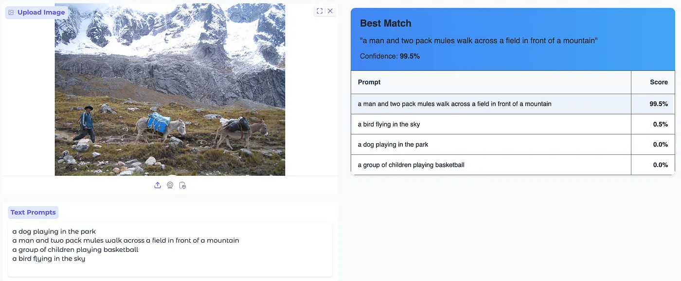
CLIP Inference with Gradio

Conclusion

In this blog, we explored the implementation of a CLIP-like model that utilizes transformer-based encoders for both images and text. We covered essential components, such as positional embeddings, multi-head attention, and transformer encoders, as well as the processes of dataset handling and tokenization. The training pipeline was specifically designed to optimize image-text alignment, while the inference function facilitated practical applications, including similarity computation and zero-shot classification.

By integrating these techniques, we developed a robust multimodal system that understands visual and textual inputs within a shared representation space. This framework can be further expanded for applications such as image retrieval, caption generation, and multimodal reasoning, highlighting the effectiveness of contrastive learning in connecting vision and language.

Thank you for reading! Happy coding!

References

• Learning Transferable Visual Models From Natural Language Supervision
• An Image is Worth 16x16 Words: Transformers for Image Recognition at Scale
• Attention is All You Need