YOLOv5 Custom Object Detection on Fashion Accessories
Table of contents
Introduction
In this project, we focused on building a custom object detection model using YOLOv5 to identify specific clothing accessories such as shirts, pants, shoes, handbags and sunglasses. The primary goal is to train a model that could accurately detect and classify above defined items in images.
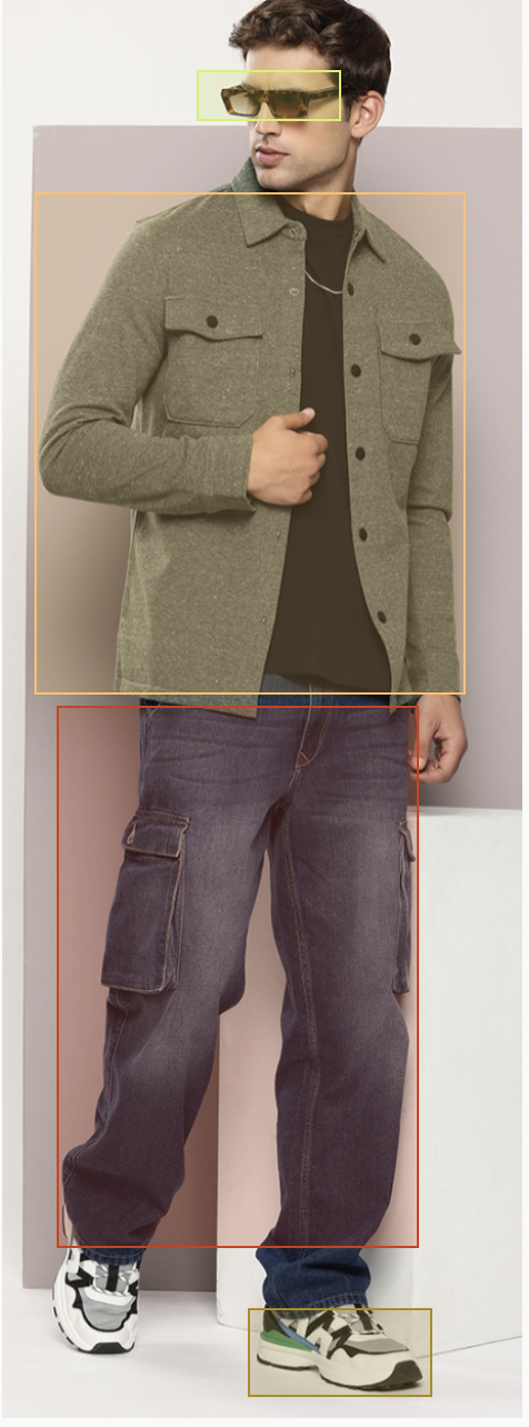
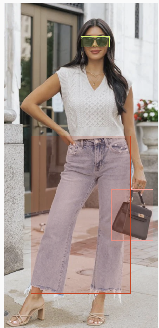
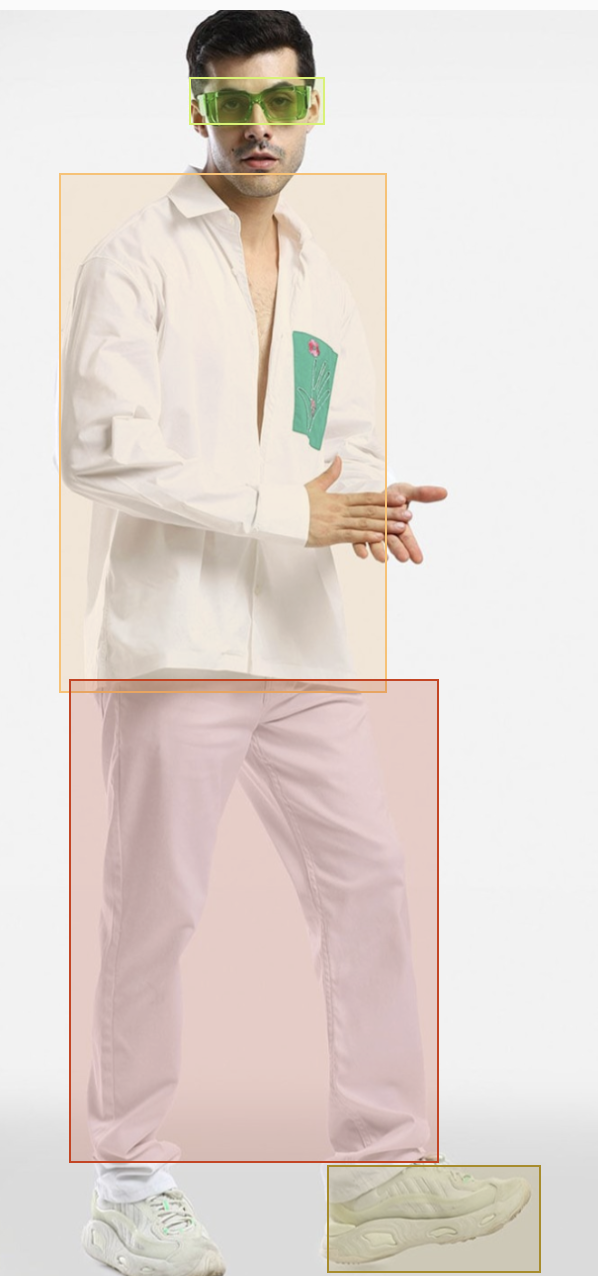
After completing the training process, we ran inference on a set of test images to evaluate the model’s performance. The results demonstrated the model’s ability to successfully identify and classify the targeted objects with high accuracy. Each detected object was marked with a bounding box, and the corresponding label was displayed.
Below are examples of the model’s output, illustrating its ability to detect and label clothing accessories:
These results validate the model’s potential for real-world applications, such as fashion analysis, e-commerce, and inventory management, where quick and precise object detection is crucial.
What is Object Detection?
Object detection is a critical task in computer vision that involves identifying and locating objects within digital images or videos. The primary goal of object detection is to answer two key questions:
-
What is the object? - Identifying category or type of an object (e.g., person, car, dog, etc.)
-
Where is the object?: determining the specific location of the object within the image or video, often represented by bounding boxes around the object.
How does object detection work?
Object detection combines two tasks:
- classification—it determines what the object is.
- localization—it identifies where the object is by drawing a bounding box around it.
Real-world use cases of object detection
- Security and Surveilleance:
- In security systems, object detection is used to monitor and identify suspicious activities.
- For instance, CCTV cameras equipped with object detection can automatically recognize unauthorized access, detect abandoned objects (e.g., luggage in airports), and alert security personnel. This improves the effectiveness of surveillance systems in places like banks, airports, and public spaces.
- Augmented Reality (AR):
- Object detection plays an important role in AR applications by enabling the interaction between digital objects and the real world.
- For example, in mobile apps like IKEA Place, object detection helps users visualize how furniture will look in their homes by detecting the room’s layout and placing virtual furniture in appropriate locations. This enhances the shopping experience by encouraging customers to try before they buy.
Object detection is a powerful tool in computer vision with a wide variety of applications across various domains.
Object Detection Algorithms
- EffcientNet:
- EfficientNet is a family of object detection models that focuses on optimizing both accuracy and efficiency.
- Built on top of the EfficientNet backbone, EfficientNet scales models architecture effectively using a compund scaling method that balances network depth, width and resolution.
- Features:
- Highly scalable
- Ideal for applications requirng high performance with limited computational resourcses.
Below is the architecture for the EfficientNet algorithm for object detection. Please read more details on EfficientNet Paper.

- SSD (Single Shot Multibox Detector):
- It processes an entire image in a single pass.
- It divides image into grid and makes predictions based on each grid cell, similar to YOLO, but with mutiple feature layers for improved accuracy.
- Features:
- Good balance between speed and accuracy
- Suitable for real-time detection on resource-constrained devices
You can find more details in the paper here.
 Architecture")
- Faster R-CNN (Region-Based CNN):
- It is a two-stage object detection algorithm that first proposes regions of interest (ROIs) and then classifies these regions into object categories.
- The first-stage involves Region Proposed Network (RPN) that generates candidate bounding boxes, and
- the second stage uses these proposals to detect the objects within them. * Features:
- High accuracy, especially for complex and cluttered scenes
- computationally intensive, requiring more processing time than YOLO
Please follow the original paper here for more details.

- YOLO (You Only Look Once):
- YOLO is one of the fastest and most efficient object detection algorithms.
- It treats object detection as a single regression problem, directly predicting the class probabilities and bounding box coordinates from an image in one evaluation.
- Unlike traditional methods that apply the image to multiple regions of an image, YOLO considers entire image at once, making it incredibly fast.
- Features:
- High speed and good accuracy
- Single forward pass through network
You can explore more details on the architecture and experiments done in the research paper here.

Here, we willbe using YOLOv5. YOLOv5 is known for its speed, accuracy and ease of use, making it a popular choice for real-time object detection.
Why YOLOv5?
-
YOLOv5 builds upon succession of previous versions of YOLO while itroducing improvements in model architecture and training techniques.
-
It offres multiple pre-trained models that vary in size and performance, allowing users to choose a model that best fits their requirements in terms of speed and accuracy.
The implementation of YOLOv5 by Ultralytics is built using PyTorch, an open-source machine learning framework. You can explore its basic through the official PyTorch Tutorial.
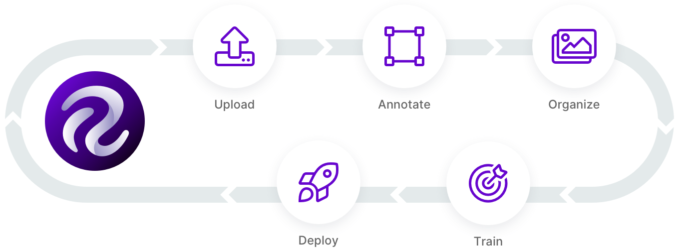
How to train YOLOv5 model?
Training a YOLOv5 model is traightforrd, thats to its user-friendly documentation. Here’s a brief overview of the steps:
-
Data Annotation
- Label your images with the necessary tags to create a dataset that the model can learn from. This labelled data is crucial for supervised machine learning.
- YOLOv5 Training
- Train a custom YOLOv5 model using the annotated dataset. After training, we’ll receive a weight file that encapsulates the learned features.
- YOLOv5 Inference
- Use the trained model to detect objects, such as clothing accessories, in new images during runtime.
1) Data Annotation
In this step, we focus on annotating the full-shot image data that has been scraped, preparing it for training a custom YOLOv5 model. Proper data annotation is crucial as it involves labeling the images with the exact locations and categories of the objects we want our model to detect.
Annotating Images in YOLOv5 Supported Format
The annotation process involves drawing bounding boxes around the target objects within the images and assigning the appropriate labels to each bounding box. For this project, we are interested in detecting specific clothing and accessories, and the labels we are considering are:
- Shirts
- Pants
- Shoes
- Handbags
- Sunglasses
Using Label Studio
To facilitate the annotation process, I used an online data annotation tool called Label Studio. Label Studio offers a user-friendly interface for drawing bounding boxes around objects and assigning labels to them, making it an efficient choice for annotating large datasets.
In the context of this project, I created bounding boxes around each instance of Handbags, Pants, Shirts, Shoes, and Sunglasses in the images. Each box was labeled accordingly, ensuring that the YOLOv5 model can later recognize these objects during training and inference.
Here’s a demo video showing the data annotation process for this project using Label Studio, which provides a visual guide on how to draw bounding boxes and assign labels effectively.
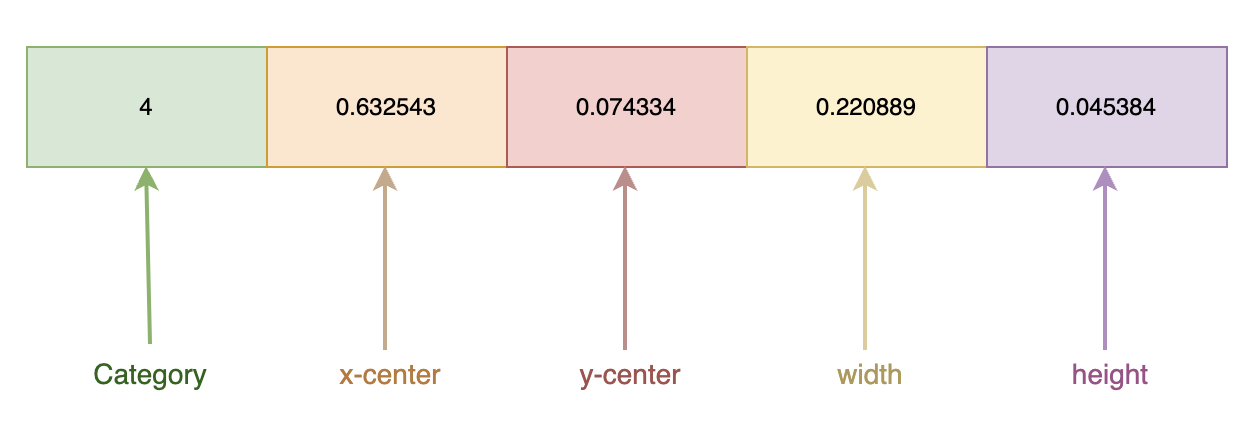
YOLOv5 Data Format
YOLOv5 requires a specific format for the annotated data, where each bounding box is stored with the following information:
- Category:
- The class or category to which the bounding box belongs (e.g., shirts, pants).
- x-center:
- The normalized X coordinate of the center of the bounding box, representing the midpoint of the object in the horizontal axis.
- y-center:
- The normalized Y coordinate of the center of the bounding box, representing the midpoint of the object in the vertical axis.
- Width:
- The normalized width of the bounding box, indicating how wide the object is relative to the image.
- Height:
- The normalized height of the bounding box, indicating how tall the object is relative to the image.
Normalization means that these coordinates and dimensions are scaled between 0 and 1, based on the size of the image. This standardization allows the YOLOv5 model to accurately process the data, regardless of the image resolution or aspect ratio.
By carefully annotating the data in this format, we ensure that the YOLOv5 model can effectively learn to detect the specified clothing and accessories during the training phase.
2) YOLOv5 Training
YOLOv5 offers five pre-defined models, each varying in size and performance. These models are:
- YOLOv5-nano
- YOLOv5-small
- YOLOv5-medium
- YOLOv5-large
- YOLOv5-extraLarge
Training the YOLOv5-Large Model
For our project, we will be training a YOLOv5 model. This model strikes a good balance between speed and accuracy, making it well-suited for our task of detecting specific clothing and accessories.
The training process will follow the steps outlined in the official YOLOv5 documentation. This documentation provides a comprehensive guide on how to train YOLOv5 models using PyTorch, including setting up the environment, preparing the dataset, and initiating the training process.
Customizing YOLOv5 for Custom Object Detection
While YOLOv5 is capable of detecting up to 80 common classes, such as cars, persons, boats, and birds, we need to customize the model to detect our specific classes: Handbags, Pants, Shirts, Shoes, and Sunglasses. To achieve this, we must create a custom .yaml file that specifies the classes we want to detect and the paths to our training and testing datasets.
.yaml File Configuration
The .yaml file is a configuration file that YOLOv5 uses to understand the structure of the dataset. Below is a general description of the key elements in the .yaml file:
-
Classes: This section lists the custom classes that we want the YOLOv5 model to detect. For our project, this would include
Handbags,Pants,Shirts,Shoes, andSunglasses. -
Train: The path to the directory containing the training images. This path tells the model where to find the images it should learn from.
-
Val (Validation): The path to the directory containing the validation images. These images are used to evaluate the model’s performance during training, ensuring that it is learning effectively.
-
Test (optional): The path to the directory containing the test images, which can be used to evaluate the model after training is complete.
Here is a snapshot of what the .yaml file might look like for our specific use case:
# Number of classes
nc: 5

# Names of the classes
names: ['Handbags', 'Pants', 'Shirts', 'Shoes', 'Sunglasses']

# Paths to the datasets
path: /content/Annotated_Data                # dataset root dir
train: /content/Annotated_Data/images/train  # train images (relative to 'path') 450 images
val: /content/Annotated_Data/images/val      # val images (relative to 'path') 50 images
test:                                        # test images (optional)

# Classes
names:
  0: Handbags
  1: Pants
  2: Shirts
  3: Shoes
  4: Sunglasses
This configuration file ensures that YOLOv5 knows exactly what classes it needs to detect and where to find the data necessary for training and validation.
By following these steps, we’ll be able to train a custom YOLOv5-large model that accurately detects the specific types of clothing and accessories we’re interested in.
Training Steps
# importing required dependencies

import pandas as pd
import numpy as np
import tensorflow as tf
import random
import cv2
from google.colab.patches import cv2_imshow
from tqdm.auto import tqdm
import os
import shutil as sh
from IPython.display import Image, clear_output
import torch
Now, we download a sample annotated dataset and use it for model training.
unzip '/content/Annotated_Data.zip'
Downloading the Ultralytics-YOLOv5 repository for training our custom YOLOv5 model using YOLOv5-large weights.
#Cloning the official YOLOv5 repository and other dependencies
git clone https://github.com/ultralytics/yolov5
pip install -U pycocotools

#Installing dependencies
pip install -qr yolov5/requirements.txt
cp yolov5/requirements.txt ./
Cloning into 'yolov5'...
remote: Enumerating objects: 16843, done.[K
remote: Counting objects: 100% (18/18), done.[K
remote: Compressing objects: 100% (18/18), done.[K
remote: Total 16843 (delta 4), reused 10 (delta 0), pack-reused 16825[K
Receiving objects: 100% (16843/16843), 15.57 MiB | 13.40 MiB/s, done.
Resolving deltas: 100% (11553/11553), done.
Requirement already satisfied: pycocotools in /usr/local/lib/python3.10/dist-packages (2.0.8)
Requirement already satisfied: matplotlib>=2.1.0 in /usr/local/lib/python3.10/dist-packages (from pycocotools) (3.7.1)
Requirement already satisfied: numpy in /usr/local/lib/python3.10/dist-packages (from pycocotools) (1.26.4)
Requirement already satisfied: contourpy>=1.0.1 in /usr/local/lib/python3.10/dist-packages (from matplotlib>=2.1.0->pycocotools) (1.2.1)
Requirement already satisfied: cycler>=0.10 in /usr/local/lib/python3.10/dist-packages (from matplotlib>=2.1.0->pycocotools) (0.12.1)
Requirement already satisfied: fonttools>=4.22.0 in /usr/local/lib/python3.10/dist-packages (from matplotlib>=2.1.0->pycocotools) (4.53.1)
Requirement already satisfied: kiwisolver>=1.0.1 in /usr/local/lib/python3.10/dist-packages (from matplotlib>=2.1.0->pycocotools) (1.4.5)
Requirement already satisfied: packaging>=20.0 in /usr/local/lib/python3.10/dist-packages (from matplotlib>=2.1.0->pycocotools) (24.1)
Requirement already satisfied: pillow>=6.2.0 in /usr/local/lib/python3.10/dist-packages (from matplotlib>=2.1.0->pycocotools) (9.4.0)
Requirement already satisfied: pyparsing>=2.3.1 in /usr/local/lib/python3.10/dist-packages (from matplotlib>=2.1.0->pycocotools) (3.1.2)
Requirement already satisfied: python-dateutil>=2.7 in /usr/local/lib/python3.10/dist-packages (from matplotlib>=2.1.0->pycocotools) (2.8.2)
Requirement already satisfied: six>=1.5 in /usr/local/lib/python3.10/dist-packages (from python-dateutil>=2.7->matplotlib>=2.1.0->pycocotools) (1.16.0)
[2K [90m━━━━━━━━━━━━━━━━━━━━━━━━━━━━━━━━━━━━━━━━[0m [32m41.3/41.3 kB[0m [31m3.1 MB/s[0m eta [36m0:00:00[0m
[2K [90m━━━━━━━━━━━━━━━━━━━━━━━━━━━━━━━━━━━━━━━━[0m [32m207.3/207.3 kB[0m [31m17.2 MB/s[0m eta [36m0:00:00[0m
[2K [90m━━━━━━━━━━━━━━━━━━━━━━━━━━━━━━━━━━━━━━━━[0m [32m4.5/4.5 MB[0m [31m101.7 MB/s[0m eta [36m0:00:00[0m
[2K [90m━━━━━━━━━━━━━━━━━━━━━━━━━━━━━━━━━━━━━━━━[0m [32m865.6/865.6 kB[0m [31m12.0 MB/s[0m eta [36m0:00:00[0m
[2K [90m━━━━━━━━━━━━━━━━━━━━━━━━━━━━━━━━━━━━━━━━[0m [32m62.7/62.7 kB[0m [31m5.6 MB/s[0m eta [36m0:00:00[0m
[?25h
We can now begin training our custom YOLOv5 object detection model. The training is expected to take some time depending on the type of hardware used.
python /content/yolov5/train.py --img 640 --batch 32 --epochs 15 --weights yolov5l.pt --data /content/Annotated_Data/pinterest.yaml
[34m[1mtrain: [0mweights=yolov5l.pt, cfg=, data=/content/Annotated_Data/pinterest.yaml, hyp=yolov5/data/hyps/hyp.scratch-low.yaml, epochs=15, batch_size=16, imgsz=640, rect=False, resume=False, nosave=False, noval=False, noautoanchor=False, noplots=False, evolve=None, evolve_population=yolov5/data/hyps, resume_evolve=None, bucket=, cache=None, image_weights=False, device=, multi_scale=False, single_cls=False, optimizer=SGD, sync_bn=False, workers=8, project=yolov5/runs/train, name=exp, exist_ok=False, quad=False, cos_lr=False, label_smoothing=0.0, patience=100, freeze=[0], save_period=-1, seed=0, local_rank=-1, entity=None, upload_dataset=False, bbox_interval=-1, artifact_alias=latest, ndjson_console=False, ndjson_file=False
[34m[1mgithub: [0mup to date with https://github.com/ultralytics/yolov5 ✅
YOLOv5 🚀 v7.0-351-g19ce9029 Python-3.10.12 torch-2.3.1+cu121 CUDA:0 (Tesla T4, 15102MiB)
[34m[1mhyperparameters: [0mlr0=0.01, lrf=0.01, momentum=0.937, weight_decay=0.0005, warmup_epochs=3.0, warmup_momentum=0.8, warmup_bias_lr=0.1, box=0.05, cls=0.5, cls_pw=1.0, obj=1.0, obj_pw=1.0, iou_t=0.2, anchor_t=4.0, fl_gamma=0.0, hsv_h=0.015, hsv_s=0.7, hsv_v=0.4, degrees=0.0, translate=0.1, scale=0.5, shear=0.0, perspective=0.0, flipud=0.0, fliplr=0.5, mosaic=1.0, mixup=0.0, copy_paste=0.0
[34m[1mComet: [0mrun 'pip install comet_ml' to automatically track and visualize YOLOv5 🚀 runs in Comet
[34m[1mTensorBoard: [0mStart with 'tensorboard --logdir yolov5/runs/train', view at http://localhost:6006/
Overriding model.yaml nc=80 with nc=5
from n params module arguments
0 -1 1 7040 models.common.Conv [3, 64, 6, 2, 2]
1 -1 1 73984 models.common.Conv [64, 128, 3, 2]
2 -1 3 156928 models.common.C3 [128, 128, 3]
3 -1 1 295424 models.common.Conv [128, 256, 3, 2]
4 -1 6 1118208 models.common.C3 [256, 256, 6]
5 -1 1 1180672 models.common.Conv [256, 512, 3, 2]
6 -1 9 6433792 models.common.C3 [512, 512, 9]
7 -1 1 4720640 models.common.Conv [512, 1024, 3, 2]
8 -1 3 9971712 models.common.C3 [1024, 1024, 3]
9 -1 1 2624512 models.common.SPPF [1024, 1024, 5]
10 -1 1 525312 models.common.Conv [1024, 512, 1, 1]
11 -1 1 0 torch.nn.modules.upsampling.Upsample [None, 2, 'nearest']
12 [-1, 6] 1 0 models.common.Concat [1]
13 -1 3 2757632 models.common.C3 [1024, 512, 3, False]
14 -1 1 131584 models.common.Conv [512, 256, 1, 1]
15 -1 1 0 torch.nn.modules.upsampling.Upsample [None, 2, 'nearest']
16 [-1, 4] 1 0 models.common.Concat [1]
17 -1 3 690688 models.common.C3 [512, 256, 3, False]
18 -1 1 590336 models.common.Conv [256, 256, 3, 2]
19 [-1, 14] 1 0 models.common.Concat [1]
20 -1 3 2495488 models.common.C3 [512, 512, 3, False]
21 -1 1 2360320 models.common.Conv [512, 512, 3, 2]
22 [-1, 10] 1 0 models.common.Concat [1]
23 -1 3 9971712 models.common.C3 [1024, 1024, 3, False]
24 [17, 20, 23] 1 53850 models.yolo.Detect [5, [[10, 13, 16, 30, 33, 23], [30, 61, 62, 45, 59, 119], [116, 90, 156, 198, 373, 326]], [256, 512, 1024]]
Model summary: 368 layers, 46159834 parameters, 46159834 gradients, 108.3 GFLOPs
Transferred 607/613 items from yolov5l.pt
[34m[1mAMP: [0mchecks passed ✅
[34m[1moptimizer:[0m SGD(lr=0.01) with parameter groups 101 weight(decay=0.0), 104 weight(decay=0.0005), 104 bias
[34m[1malbumentations: [0mBlur(p=0.01, blur_limit=(3, 7)), MedianBlur(p=0.01, blur_limit=(3, 7)), ToGray(p=0.01), CLAHE(p=0.01, clip_limit=(1, 4.0), tile_grid_size=(8, 8))
[34m[1mtrain: [0mScanning /content/Annotated_Data/labels/train.cache... 450 images, 0 backgrounds, 0 corrupt: 100% 450/450 [00:00<?, ?it/s]
/usr/lib/python3.10/multiprocessing/popen_fork.py:66: RuntimeWarning: os.fork() was called. os.fork() is incompatible with multithreaded code, and JAX is multithreaded, so this will likely lead to a deadlock.
self.pid = os.fork()
[34m[1mval: [0mScanning /content/Annotated_Data/labels/val.cache... 50 images, 0 backgrounds, 0 corrupt: 100% 50/50 [00:00<?, ?it/s]
[34m[1mAutoAnchor: [0m4.66 anchors/target, 0.996 Best Possible Recall (BPR). Current anchors are a good fit to dataset ✅
Plotting labels to yolov5/runs/train/exp2/labels.jpg...
Image sizes 640 train, 640 val
Using 2 dataloader workers
Logging results to [1myolov5/runs/train/exp2[0m
Starting training for 15 epochs...
Epoch GPU_mem box_loss obj_loss cls_loss Instances Size
0/14 9.85G 0.09428 0.05607 0.04508 9 640: 100% 29/29 [00:46<00:00, 1.61s/it]
Class Images Instances P R mAP50 mAP50-95: 100% 2/2 [00:08<00:00, 4.21s/it]
all 50 149 0.757 0.211 0.187 0.0464
Epoch GPU_mem box_loss obj_loss cls_loss Instances Size
1/14 10.3G 0.06949 0.05329 0.02564 14 640: 100% 29/29 [00:41<00:00, 1.42s/it]
Class Images Instances P R mAP50 mAP50-95: 100% 2/2 [00:01<00:00, 1.20it/s]
all 50 149 0.457 0.589 0.401 0.107
Epoch GPU_mem box_loss obj_loss cls_loss Instances Size
2/14 10.3G 0.06675 0.04398 0.01508 16 640: 100% 29/29 [00:44<00:00, 1.53s/it]
Class Images Instances P R mAP50 mAP50-95: 100% 2/2 [00:01<00:00, 1.57it/s]
all 50 149 0.26 0.485 0.328 0.103
Epoch GPU_mem box_loss obj_loss cls_loss Instances Size
3/14 10.3G 0.06548 0.03972 0.01043 15 640: 100% 29/29 [00:42<00:00, 1.48s/it]
Class Images Instances P R mAP50 mAP50-95: 100% 2/2 [00:01<00:00, 1.26it/s]
all 50 149 0.282 0.704 0.537 0.177
Epoch GPU_mem box_loss obj_loss cls_loss Instances Size
4/14 10.3G 0.06062 0.03606 0.00862 12 640: 100% 29/29 [00:41<00:00, 1.44s/it]
Class Images Instances P R mAP50 mAP50-95: 100% 2/2 [00:01<00:00, 1.38it/s]
all 50 149 0.404 0.798 0.667 0.328
Epoch GPU_mem box_loss obj_loss cls_loss Instances Size
5/14 10.3G 0.05276 0.03419 0.007469 13 640: 100% 29/29 [00:43<00:00, 1.51s/it]
Class Images Instances P R mAP50 mAP50-95: 100% 2/2 [00:01<00:00, 1.43it/s]
all 50 149 0.514 0.609 0.582 0.328
Epoch GPU_mem box_loss obj_loss cls_loss Instances Size
6/14 10.3G 0.04568 0.03347 0.005993 7 640: 100% 29/29 [00:43<00:00, 1.50s/it]
Class Images Instances P R mAP50 mAP50-95: 100% 2/2 [00:02<00:00, 1.18s/it]
all 50 149 0.514 0.772 0.6 0.334
Epoch GPU_mem box_loss obj_loss cls_loss Instances Size
7/14 10.3G 0.0409 0.03169 0.004739 6 640: 100% 29/29 [00:44<00:00, 1.54s/it]
Class Images Instances P R mAP50 mAP50-95: 100% 2/2 [00:02<00:00, 1.12s/it]
all 50 149 0.676 0.826 0.786 0.493
Epoch GPU_mem box_loss obj_loss cls_loss Instances Size
8/14 10.3G 0.0381 0.03034 0.00471 7 640: 100% 29/29 [00:41<00:00, 1.42s/it]
Class Images Instances P R mAP50 mAP50-95: 100% 2/2 [00:01<00:00, 1.37it/s]
all 50 149 0.863 0.888 0.902 0.52
Epoch GPU_mem box_loss obj_loss cls_loss Instances Size
9/14 10.3G 0.035 0.02909 0.004154 22 640: 100% 29/29 [00:42<00:00, 1.45s/it]
Class Images Instances P R mAP50 mAP50-95: 100% 2/2 [00:01<00:00, 1.46it/s]
all 50 149 0.81 0.863 0.87 0.515
Epoch GPU_mem box_loss obj_loss cls_loss Instances Size
10/14 10.3G 0.03239 0.02947 0.003605 11 640: 100% 29/29 [00:42<00:00, 1.47s/it]
Class Images Instances P R mAP50 mAP50-95: 100% 2/2 [00:01<00:00, 1.40it/s]
all 50 149 0.828 0.872 0.869 0.571
Epoch GPU_mem box_loss obj_loss cls_loss Instances Size
11/14 10.3G 0.03016 0.02709 0.003643 9 640: 100% 29/29 [00:42<00:00, 1.48s/it]
Class Images Instances P R mAP50 mAP50-95: 100% 2/2 [00:01<00:00, 1.43it/s]
all 50 149 0.822 0.896 0.893 0.628
Epoch GPU_mem box_loss obj_loss cls_loss Instances Size
12/14 10.3G 0.02786 0.02756 0.003469 11 640: 100% 29/29 [00:41<00:00, 1.42s/it]
Class Images Instances P R mAP50 mAP50-95: 100% 2/2 [00:01<00:00, 1.53it/s]
all 50 149 0.87 0.862 0.9 0.619
Epoch GPU_mem box_loss obj_loss cls_loss Instances Size
13/14 10.3G 0.02609 0.02607 0.002858 14 640: 100% 29/29 [00:46<00:00, 1.61s/it]
Class Images Instances P R mAP50 mAP50-95: 100% 2/2 [00:01<00:00, 1.40it/s]
all 50 149 0.859 0.886 0.9 0.632
Epoch GPU_mem box_loss obj_loss cls_loss Instances Size
14/14 10.3G 0.02503 0.02679 0.00295 15 640: 100% 29/29 [00:42<00:00, 1.48s/it]
Class Images Instances P R mAP50 mAP50-95: 100% 2/2 [00:01<00:00, 1.38it/s]
all 50 149 0.853 0.889 0.907 0.649
15 epochs completed in 0.220 hours.
Optimizer stripped from yolov5/runs/train/exp2/weights/last.pt, 92.8MB
Optimizer stripped from yolov5/runs/train/exp2/weights/best.pt, 92.8MB
Validating yolov5/runs/train/exp2/weights/best.pt...
Fusing layers...
Model summary: 267 layers, 46129818 parameters, 0 gradients, 107.7 GFLOPs
Class Images Instances P R mAP50 mAP50-95: 100% 2/2 [00:02<00:00, 1.14s/it]
all 50 149 0.854 0.889 0.907 0.649
Handbags 50 10 0.73 0.9 0.839 0.683
Pants 50 45 0.94 0.933 0.978 0.807
Shirts 50 32 0.842 0.938 0.92 0.744
Shoes 50 41 0.758 0.683 0.805 0.527
Sunglasses 50 21 1 0.992 0.995 0.482
Results saved to [1myolov5/runs/train/exp2[0m
we will be using tensorboard for data logging during model training.
from tensorboard import notebook

%load_ext tensorboard
%tensorboard --logdir /content/yolov5/runs/train

notebook.display(port=6006, height=1000)
Selecting TensorBoard with logdir /content/yolov5/runs/train (started 0:00:00 ago; port 6006, pid 8519).
# Converting the weights from .pt format to .onnx format
python yolov5/export.py --weights  /content/yolov5/runs/train/exp2/weights/best.pt --include onnx
[34m[1mexport: [0mdata=yolov5/data/coco128.yaml, weights=['/content/yolov5/runs/train/exp2/weights/best.pt'], imgsz=[640, 640], batch_size=1, device=cpu, half=False, inplace=False, keras=False, optimize=False, int8=False, per_tensor=False, dynamic=False, simplify=False, mlmodel=False, opset=17, verbose=False, workspace=4, nms=False, agnostic_nms=False, topk_per_class=100, topk_all=100, iou_thres=0.45, conf_thres=0.25, include=['onnx']
YOLOv5 🚀 v7.0-351-g19ce9029 Python-3.10.12 torch-2.3.1+cu121 CPU
Fusing layers...
Model summary: 267 layers, 46129818 parameters, 0 gradients, 107.7 GFLOPs
[34m[1mPyTorch:[0m starting from /content/yolov5/runs/train/exp2/weights/best.pt with output shape (1, 25200, 10) (88.5 MB)
[34m[1mONNX:[0m starting export with onnx 1.16.2...
[34m[1mONNX:[0m export success ✅ 5.1s, saved as /content/yolov5/runs/train/exp2/weights/best.onnx (176.4 MB)
Export complete (9.0s)
Results saved to [1m/content/yolov5/runs/train/exp2/weights[0m
Detect: python detect.py --weights /content/yolov5/runs/train/exp2/weights/best.onnx
Validate: python val.py --weights /content/yolov5/runs/train/exp2/weights/best.onnx
PyTorch Hub: model = torch.hub.load('ultralytics/yolov5', 'custom', '/content/yolov5/runs/train/exp2/weights/best.onnx')
Visualize: https://netron.app
We have now successfully trained our custom YOLOv5s model. We will now save the model weights and use it for inference
# Downloading the exported weight
from google.colab import files
files.download('/content/yolov5/runs/train/exp2/weights/best.onnx')
3) YOLOv5 Inference
In this step, we’ll use the trained YOLOv5 model to run inference on test images, utilizing the saved weights from the training process. The goal is to accurately identify and classify various clothing accessories, such as shirts, pants, shoes, handbags, and sunglasses in new images.
Running Inference with OpenCV-DNN
To perform inference, we’ll utilize OpenCV-DNN (Deep Neural Network module in OpenCV), which provides an efficient way to load and run the YOLOv5 model on images. OpenCV-DNN is a popular tool for deploying deep learning models, offering high performance and compatibility with different programming languages like Python and C++.
Using OpenCV-DNN with our custom YOLOv5-small model, we can detect and classify objects in images, highlighting them with bounding boxes and labels. This approach is particularly useful for real-time applications where speed and accuracy are essential.
You can find more detailed guidance on how to implement YOLOv5 inference using OpenCV-DNN in the official OpenCV-DNN documentation. This resource provides step-by-step instructions for setting up the environment, loading the YOLOv5 model, and running inference on images, whether you are working with Python or C++.
# importing necessary dependencies
import cv2
import time
import sys
import numpy as np
import os

from matplotlib import pyplot as plt
# width of an image
INPUT_WIDTH = 640

# height of an image
INPUT_HEIGHT = 640

# confidence threshold for object detection
CONFIDENCE_THRESHOLD = 0.5

# making an array of all categories
CATEGORIES = ['Handbags', 'Pants', 'Shirts', 'Shoes', 'Sunglasses']
# load model using OpenCV
def build_model():
  # load custom YOLOv5
  model = cv2.dnn.readNet('/content/best.onnx')
  # return loaded model
  return model
# performing object detection
def detect(image, net):
  # convert image to blob
  # mean subtraction and scaling
  blob = cv2.dnn.blobFromImage(image, 1/255.0,
                            (INPUT_WIDTH, INPUT_HEIGHT),
                            swapRB=True, crop=False)

  # set the blob as input to the network
  net.setInput(blob)

  # get prediction from the model
  prediction = net.forward()
  return prediction
# load classes
class_list = CATEGORIES
class_list
['Handbags', 'Pants', 'Shirts', 'Shoes', 'Sunglasses']
# pre-processing
def format_yolov5(frame):

  # defining number of rows and columns in image numpy representation
  row, col, _ = frame.shape

  # finding the maximum between row and column
  _max = max(col, row)

  # initializing result matrix with zeros
  result = np.zeros((_max, _max, 3), np.uint8)

  # copying data from frame ndarray to result
  result[0:row, 0:col] = frame

  return result
# post-preprocessing
def wrap_detection(input_image, output_data):
  class_ids = []
  confidences = []
  boxes = []

  # fetching number of rows in output_data
  rows = output_data.shape[0]

  # fetching width and height of input_image
  image_width, image_height, _ = input_image.shape

  # x-factor for resizing
  x_factor = image_width / INPUT_WIDTH

  # y_factor for resizing
  y_factor =  image_height / INPUT_HEIGHT

  # iterate through detections
  for r in range(rows):

    # fetch bounding box co-ordinates
    row = output_data[r]

    # fetch confidence of the detection
    confidence = row[4]

    # filitering out good detections
    if confidence >= CONFIDENCE_THRESHOLD:
      classes_scores = row[5:]

      # get index of max class score
      _, _, _, max_idx = cv2.minMaxLoc(classes_scores)
      class_id = max_idx[1]

      if (classes_scores[class_id] > 0.25):
        # append confidence of new bounding box to the list
        confidences.append(confidence)
        class_ids.append(class_id)

        # get coordinated center (x and y) and width and height of the bounding box
        x, y, w, h = row[0].item(), row[1].item(), row[2].item(), row[3].item()

        # calculate x-coordinate of top-left point of bounding box
        left = int((x-0.5*w) * x_factor)

        # calculate y-coordinate of top-left point of bounding box
        top = int((y-0.5*h) * y_factor)

        # calculate width of bounding box
        width = int(w * x_factor)

        # calculate height of bounding box
        height = int(h * y_factor)

        # create array of coordinates of the bounding box
        box = np.array([left, top, width, height])
        # append new bounding box coordinates to the list
        boxes.append(box)

  # use non-maximum suppression to avoid multiple bounding boxes for the same object
  indexes = cv2.dnn.NMSBoxes(boxes, confidences, 0.25, 0.45)

  # define new lists to store class ID's, confidences and bounding boxes
  result_class_ids = []
  result_confidences = []
  result_boxes = []

  # loop through indices
  for i in indexes:
    # add detection confidence to the list
    result_confidences.append(confidences[i])

    # add detection class id to the list
    result_class_ids.append(class_ids[i])

    # add detection bounding box to the list
    result_boxes.append(boxes[i])

  return result_class_ids, result_confidences, result_boxes
# define colors for drawing bounding boxes
colors = [(255, 255, 0), (0, 255, 0), (0, 255, 255), (255, 0, 0), (255, 0, 255)]

# load model for inference
net = build_model()
import cv2
from matplotlib import pyplot as plt

def display_object_detection(frame):
    # Display the input and detected images
    plt.figure(figsize=(8, 8))
    # Show the detected image
    plt.imshow(cv2.cvtColor(frame, cv2.COLOR_BGR2RGB))
    plt.title('YOLOv5 Detection')
    plt.axis('off')
    plt.show()

# Main function for the custom object detection
def yolo_detect(img_path):
    # Read the image
    frame = cv2.imread(img_path)
    # Proceed forward if the image read above is not None
    if frame is not None:

        # Make a copy of the original image for displaying later
        original_image = frame.copy()

        # Pre-process the input image
        inputImage = format_yolov5(frame)
        # Object detection using our custom model
        outs = detect(inputImage, net)

        # Post-process the detections
        class_ids, confidences, boxes = wrap_detection(inputImage, outs[0])

        # Iterate through the detections for drawing annotations on the image
        for (classid, confidence, box) in zip(class_ids, confidences, boxes):
            # Choosing the color for drawing annotations
            color = colors[int(classid) % len(colors)]
            # Drawing the bounding box
            cv2.rectangle(frame, box, color, 2)
            # Preparing the label with class name and confidence score
            label = f"{class_list[classid]}"
            # Calculating label size
            label_size, base_line = cv2.getTextSize(label, cv2.FONT_HERSHEY_SIMPLEX, 0.5, 1)
            # Drawing a filled rectangle above the bounding box for the label
            top_left = (box[0], box[1] - label_size[1] - base_line)
            bottom_right = (box[0] + label_size[0], box[1])
            cv2.rectangle(frame, top_left, bottom_right, color, cv2.FILLED)
            # Writing the label on top of the bounding box
            cv2.putText(frame, label, (box[0], box[1] - base_line), cv2.FONT_HERSHEY_SIMPLEX, 0.5, (0, 0, 0), 1)

        # Save the annotated image
        annotated_img_path = 'annotated_' + img_path.split('/')[-1]
        cv2.imwrite(annotated_img_path, frame)

        # display_object_detection(frame)
        return annotated_img_path
yolo_detect('input1.png')
yolo_detect('input2.png')
yolo_detect('input3.png')
Now, we will do the inference on more input itest mages to see how the object detection performs.
import cv2
import os
from matplotlib import pyplot as plt

# Function to create a grid of images
def create_image_grid(image_list, grid_size):
    # Calculate the size of the grid
    grid_rows, grid_cols = grid_size, grid_size
    fig, axes = plt.subplots(grid_rows, grid_cols, figsize=(15, 15))
    fig.subplots_adjust(hspace=0.1, wspace=0.05)

    # Iterate over the images and add them to the grid
    for i, img_path in enumerate(image_list):
        # Read the image
        frame = cv2.imread(img_path)
        if frame is not None:
            # Perform object detection and get the annotated image
            annotated_img_path = yolo_detect(img_path)
            # Read the annotated image
            detected_img = cv2.imread(annotated_img_path)
            # Convert BGR to RGB for displaying
            detected_img_rgb = cv2.cvtColor(detected_img, cv2.COLOR_BGR2RGB)

            # Calculate the row and column in the grid
            row = i // grid_cols
            col = i % grid_cols
            # Plot the image on the grid
            axes[row, col].imshow(detected_img_rgb)
            axes[row, col].axis('off')

    plt.show()

# Function to process a directory of images
def process_dir(directory_path, grid_size=(3, 3)):
    image_list = [os.path.join(directory_path, img) for img in os.listdir(directory_path) if img.endswith(('.jpg', '.png', '.jpeg'))]

    # Ensure that all images are resized to the same dimensions
    annotated_images = [yolo_detect(img) for img in image_list]

    # Create a grid of the processed images
    create_image_grid(annotated_images, grid_size[0])
process_dir('input')
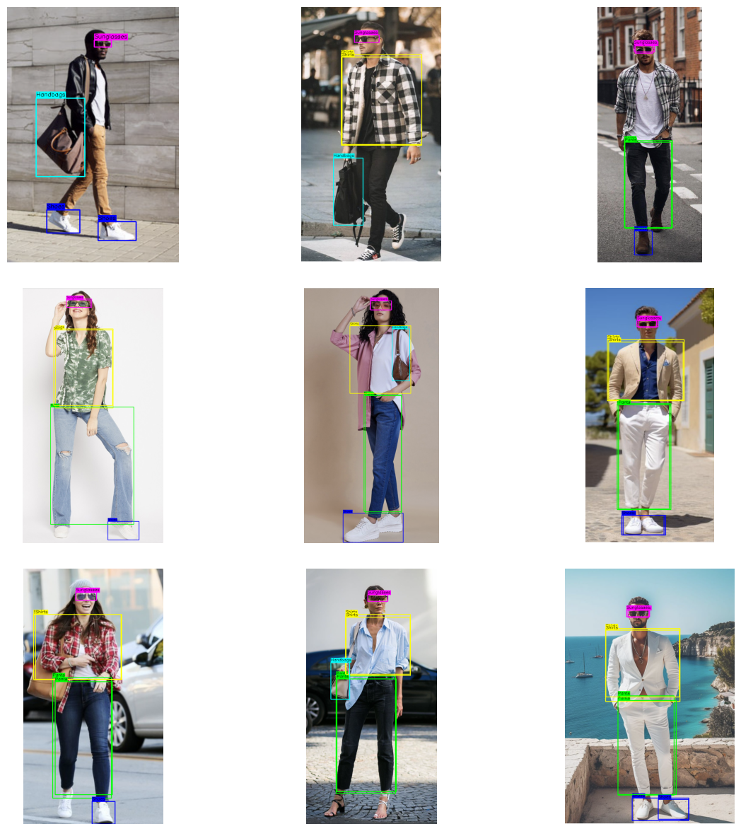
In this project, we successfully trained a model for custom object detection that can identify and detect clothing accessories like topwear, bottomwear, eyewear, footwear, and handbags worn by individuals. The model has been fine-tuned to accurately locate and label these accessories in images, which is helpful in applications such as fashion analysis and personal styling.